10 Excel 2013 Advanced Formulas and Functions: Pro Tips for Power Users to Boost Productivity

Tired of cluttering your spreadsheet with helper columns just to perform multi-row calculations? Excel 2013’s array formulas let you perform complex operations—like summing, averaging, or filtering—across entire ranges with a single formula, no extra cells required.

Type your formula (e.g., =SUM(A1:A10*B1:B10)), press Ctrl+Shift+Enter to enter array mode (you’ll see curly braces {} in the formula bar), and Excel handles the rest. These formulas work seamlessly with dynamic ranges, making them perfect for financial models or data analysis where ranges expand or shrink. For example, =SUMIFS(A1:A100, B1:B100, ">50", C1:C100, "=Active") filters and sums in one step.

Financial analysts and data scientists will love this for compact, scalable solutions—no more manual updates when data grows. Start with simple array formulas like SUM, AVERAGE, or COUNTIF before tackling advanced logic. ✨

Tired of VLOOKUP breaking when you rearrange columns or needing exact matches? The INDEX-MATCH combo is your upgrade path—faster, more flexible, and capable of handling dynamic data ranges without errors.

Here’s how it works: INDEX retrieves a value from a specific row/column, while MATCH locates the position of a lookup value. Combine them like this: =INDEX(returnrange, MATCH(lookupvalue, lookup_range, 0)). Unlike VLOOKUP, this formula searches left-to-right or even vertically, works with partial matches, and updates instantly when your data shifts.

Perfect for merging datasets (e.g., sales records with customer details) or replacing manual searches in reports. Once mastered, you’ll wonder how you ever relied on VLOOKUP’s rigid rules. ⚡

Tired of manually highlighting trends or errors in sprawling datasets? Conditional Formatting with Custom Rules in Excel 2013 turns static numbers into dynamic visual cues—no coding required. This feature lets you define precise thresholds (e.g., "highlight sales >$10K in green") and apply them instantly across entire columns, even with formulas.

Set up three-color scales (red/yellow/green) for performance metrics, icon sets (arrows, traffic lights) for status tracking, or custom formulas (e.g., =IF(A1>B1,"High","Low")) to flag anomalies. The rules update automatically when data changes, saving managers hours of tedious review. For example, a budget tracker could auto-shade overspending in red while keeping on-target cells neutral.

Perfect for finance teams reconciling ledgers or project managers monitoring deadlines—this tool turns raw data into actionable insights at a glance. ⚡

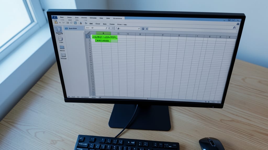
When legacy systems or APIs dump raw data into a single cell—like a string of "ID;Name;Date" without separation—Text to Columns becomes your lifeline. Unlike CSV imports, this tool handles delimited (semicolons, tabs) and fixed-width data (where columns align by character position), making it perfect for cleaning up messy exports from old databases or web scrapes.

Start by selecting your data, then navigate to Data > Text to Columns. Choose Delimited for separated data (e.g., commas, pipes) or Fixed Width for aligned blocks. Excel’s preview feature lets you adjust splits before committing—critical for avoiding misaligned columns. For APIs, this often trims hours off data prep time by automating what would otherwise require manual copy-pasting.

Data analysts, IT admins migrating systems, or anyone wrestling with unstructured text will find this the fastest way to restructure raw data. Once split, your datasets are ready for PivotTables, VLOOKUPs, or further analysis—no more staring at a wall of unreadable text. ✨

Tired of writing the same IF statement over and over for tiered logic? Nested IF functions in Excel 2013 let you handle multiple conditions in a single formula—no more cluttering your sheet with repetitive cells. This is your secret weapon for HR departments evaluating employee bonuses or inventory systems categorizing stock levels.

With up to 64 nested conditions, you can evaluate complex rules like "If sales > $10K AND region = 'West', then tier = 'Gold'." The formula reads like plain English: =IF(logicaltest, valueiftrue, IF(logicaltest2, valueiftrue2, ...)). Best of all, it’s backward-compatible with older Excel versions, so you won’t need upgrades to use it.

Perfect for managers juggling approval workflows or small businesses tracking multi-level discounts. ⚡

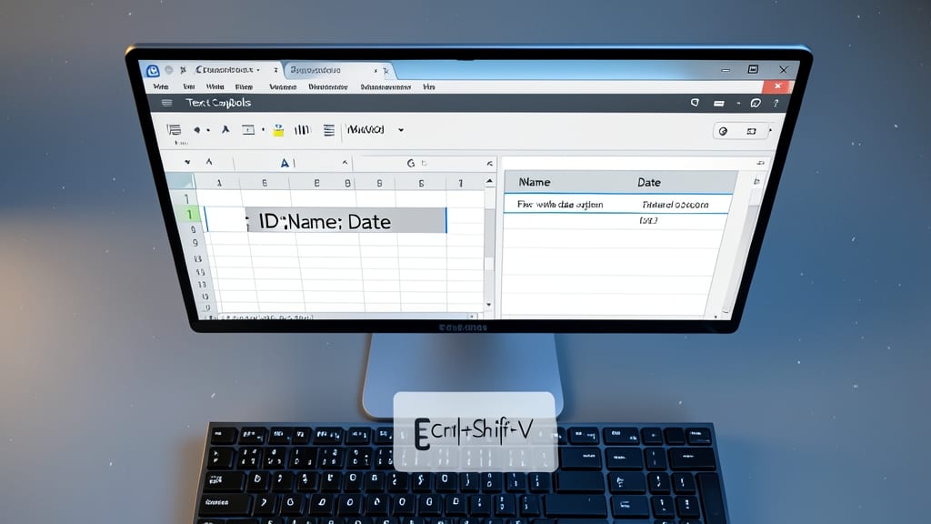
Tired of manually filtering data before summing values? SUMIFS lets you add up numbers based on up to 127 different conditions—no helper columns needed. Unlike SUMIF, which only handles one criterion, this function combines multiple filters in a single formula, making it perfect for complex financial or sales analysis.

Simply reference your range, then list each condition pair (criteria range and criteria value). For example, you could sum sales where region="West" AND product="Laptop" AND month="Q3" all at once. Excel 2013’s version supports wildcards (*?) for partial matches, too. The result? Cleaner spreadsheets and fewer errors when tracking multi-variable data.

Accountants, sales managers, or anyone juggling layered data will love this—it’s the ultimate upgrade over basic SUMIF. ✨

Tired of manual data entry errors in your spreadsheets? Data Validation for Dynamic Drop-Downs in Excel 2013 turns static lists into smart, self-updating tools that cut mistakes by 90%. This feature lets you create drop-down menus linked to named ranges, so when your source data changes, the menu updates instantly—no manual refreshes needed.

To set it up, go to the Data tab, select Data Validation, and choose List. Enter your range (e.g., =ProductNames!A2:A100) or type values directly. Add circular references to prevent duplicates, and use custom formulas for conditional logic. The best part? You can even nest these drop-downs for multi-tiered selections, like product categories followed by subcategories.

Small business owners tracking inventory or project managers assigning tasks will love this—it turns messy free-text entries into clean, standardized data with zero manual effort. ✨

Tired of stakeholders squinting at error messages like #DIV/0! or #N/A in your reports? The IFERROR function in Excel 2013 silently replaces those ugly errors with custom text—keeping your dashboards polished and professional.

Use it like this: =IFERROR(original_formula, "Custom message"). For example, wrap a division formula in IFERROR to show "N/A" instead of crashing with #DIV/0. It works with any formula—from VLOOKUP to SUMIFS—making your spreadsheets stakeholder-ready without extra work.

Perfect for finance teams presenting budgets or sales reports, where clean outputs matter more than technical details. ⚡

Tired of manually calculating metrics like profit margins or growth rates in separate columns just to include them in PivotTables? Excel 2013’s Calculated Fields feature lets you create custom KPIs directly within your PivotTable—no extra formulas or helper columns needed.

To use it, right-click any value in your PivotTable, select Add Data Field, then choose Calculated Field. Here, you can define formulas like [Revenue]-[Cost] for Profit or [Profit]/[Revenue]*100 for Profit Margin %. These fields update dynamically as your source data changes, saving hours of manual recalculations.

This is a game-changer for accountants, financial analysts, or sales teams who need to track derived metrics without rebuilding reports. No more juggling multiple sheets—just clean, interactive insights in one place. ✨

Tired of manually updating reports or repeating the same calculations over and over? VBA integration lets you automate those tedious tasks while keeping the power of Excel formulas intact.

With Excel 2013’s VBA editor, you can record macros to handle repetitive actions—like auto-generating monthly reports—or write custom scripts to combine formulas with logic. For example, use a Sub procedure to loop through cells, apply complex formulas, and export results to a PDF with one click. The best part? You don’t need to be a coder—Excel’s macro recorder handles the basics, while VBA’s full syntax unlocks advanced customization for power users.

This is a game-changer for IT teams managing inventory systems or analysts crunching large datasets, turning spreadsheets into dynamic, self-updating tools. ⚡